
 In a number of earlier posts we have talked about the shortcomings of current database technologies and query languages and how they prevent us from building systems that are capable of asking and answering complex ‘knowledge level‘ queries and above. Ultimately of course it is exactly these kinds of complex questions that we seek to answer. In this post I want to examine how one actually asks such questions in a Mitopia® environment, and show how radically the approach differs from a much simpler traditional (e.g., SQL query) scenario. Other future posts will look at the question of how Mitopia® executes these queries, for now we will focus just on the process of ‘asking’ the question through a GUI interface.
NOTE:You will find demos involving link analysis based queries in the “Mitopia.demo.m4v” (go to offset 22:40) and “MitopiaBigData.mov” (go to offset 11:20) videos on the “Videos,demos & papers” page. For a detailed look at other complex query types, see the “MitoipaNoSQL.m4v” video on the same page.
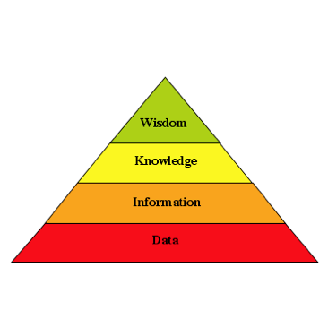 Before we proceed, we must first compare and contrast the kinds of questions that one can ask of a ‘database’ depending on the underlying organizational data model. The knowledge pyramid (shown to the right) serves as a common classification for the levels of data organization and also for the types of questions that can potentially be asked and answered by data organized at that level.
The ‘data’ level can be characterized in this context as being based on a ‘document model’, that is queries are limited to something like ‘find me all documents containing the following words’, there is no detailed structure that can be queried through the query language. The world wide web and issuing a Google query is the classic example of this very primitive level of query. The results come back as millions of document hits, and the user must read some of the documents and figure out for themselves if the answer to their original question (which of course they had to pose as a series of key words) is anywhere within the set.
The ‘information’ level corresponds to organizing data into a set of tables which can be queried as to the content of table fields (i.e., a taxonomy) – in other words this is the domain of relational databases and the standard SQL query language. Because the underlying data model is more detailed, one can ask somewhat more complex questions of the general class “find me all records where field ‘A’ has value ‘a’ and/or field ‘B’ has value ‘b'”. The SQL language allows Boolean conditions and text/numeric operators to be applied to appropriate fields. Information-level queries in general allow one to ask about the content of fields within a table, however it is difficult (i.e., requires a ‘join‘) or impossible to ask questions about the ‘connections’ between things in a data set, particularly if the schema was not designed up front to answer that particular question. This makes relational databases great for answering questions about record content and transactions in tightly constrained domains (e.g., a bank account), but pretty much useless for asking questions about the real world and the things going on within it (a very un-constrained connection-based domain).
In this particular post we will ignore ‘wisdom’ level queries and focus on ‘knowledge’ level queries, i.e., queries based not just on the content of records, but also on the many (indirect and changing) relationships between records of a wide variety of types. There is no existing standard query language that handles this level of query since these questions require a contiguous ontology (of everything) as the underpinnings for the database. We have discussed these underpinnings in previous posts, now we will explain how a user is able to easily ask these questions. These kinds of questions might be characterized as in the class “find me all records having a direct (or highly indirect but) ‘significant’ relationship to another entity/concept”. For example, one might ask “Find me all people who might potentially be running or setting up a methamphetamine lab”, “How does this disaster impact my stock portfolio”, or perhaps “Find me all passengers on a plane that may have links to terrorism”. These questions and others like them are exactly those that people really have in mind when they pose queries, yet it is clearly impossible to ask, let alone answer such questions with an ‘information’ or ‘data’ level substrate. In Mitopia® such queries can be posed directly and easily.
It is assumed below that the reader is already familiar with Mitopia’s Carmot ontology, with the basics of the MitoPlex™/MitoQuest™ federation, and with Mitopia’s approach to auto-generating the GUI.
Mitopia’s Link Analysis tool
 First let us examine Mitopia’s link analysis tool and how it is used to explore the links between persistent data items as mediated through all item types by the underlying Carmot ontology. Link analysis is conventionally a process of visualizing data and connections within it so that the the analyst can grasp a larger picture, it has nothing to do with query or predictive detection, but is instead a means to represent past data in a way the human analyst can more easily interpret. A conventional example (from Centrifuge Systems) is shown to the left. As we will see below, Mitopia®, through its contiguous ontology approach, takes this process to an entirely different level that includes both query and continuous/predictive monitoring. The screen shot below shows Mitopia’s ‘shortest path‘ link analysis tool in use:
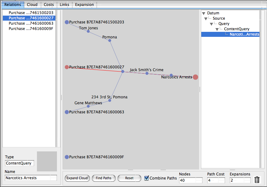
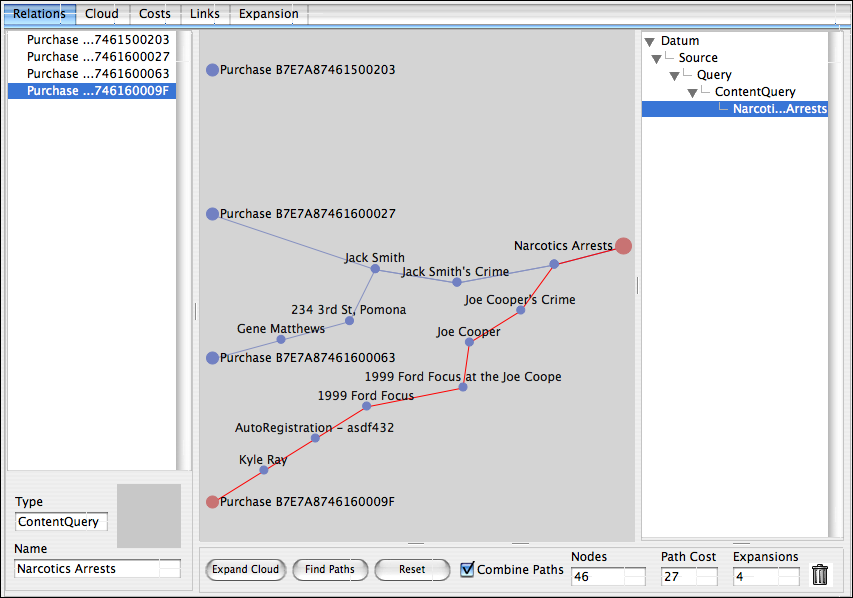
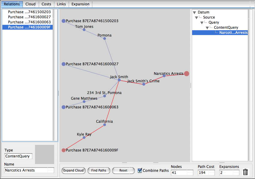
The scenario above is that of a police department looking for anybody that may be operating a methamphetamine lab. One of the essential precursors for meth is pseudoephedrine (PSE) which is commonly used in decongestants, and which as a result must now be purchased at the pharmacy counter and requires the purchaser to identify themselves. In this scenario, we have chosen to begin exploring this question by looking for connections between people purchasing PSE (assuming the police department receives a ‘feed’ of such purchases from pharmacies), and anyone that the department has arrested in the past for narcotics crimes (a data set that the police department obviously possesses). The endpoints on the left of the central ‘path’ area are four different reported PSE purchases that we will use to train the link analyzer, the single endpoint on the right is a Mitopia® query for all persons arrested in the past for narcotics crimes. These endpoints were simply dragged and dropped into the link analyzer, and could be any type (or combination of types) described by the ontology. In the state depicted above, the user has expanded the ‘cloud’ of potential connections from the training data (on the left) to the target concept (on the right) by clicking the ‘Expand Cloud’ button (twice) and then the ‘Find Paths’ button. As can be seen, the system has found a connection between all four purchases, and the individual ‘Jack Smith’ who was earlier arrested for narcotics violations. In this case the user has selected the fourth purchase and the system is highlighting the total ‘path cost’ to get from that source to the endpoint on the right hand side (in this case 194). The shortest path visualizer works by training the system which kinds of links are important (i.e., have low cost), and which are not (i.e., have high cost), so that ultimately the shortest paths show will be those that are of particular significance to the problem at hand.
Starting with the second purchase from the top, we can see that this corresponds to ‘Jack Smith’ himself purchasing PCE (total path cost = 4). Either Jack has a snotty nose, or he is not the sharpest tool in the shed. Regardless, this is clearly a significant, if very simple connection that we would want the system to detect. No need to tweak anything for this connection then.
However, if we look at the highlighted path, we see that it passes through a total of six links to make the connection starting with another individual ‘Kyle Ray’ (the purchaser) and then going through the State of California! This looks like a link that should not be considered ‘significant’. To investigate the reasons for this connection, we double click on ‘Kyle Ray’ in the diagram which then displays the ‘Links’ tab (as opposed to the initial ‘Relations’ tab) as follows:
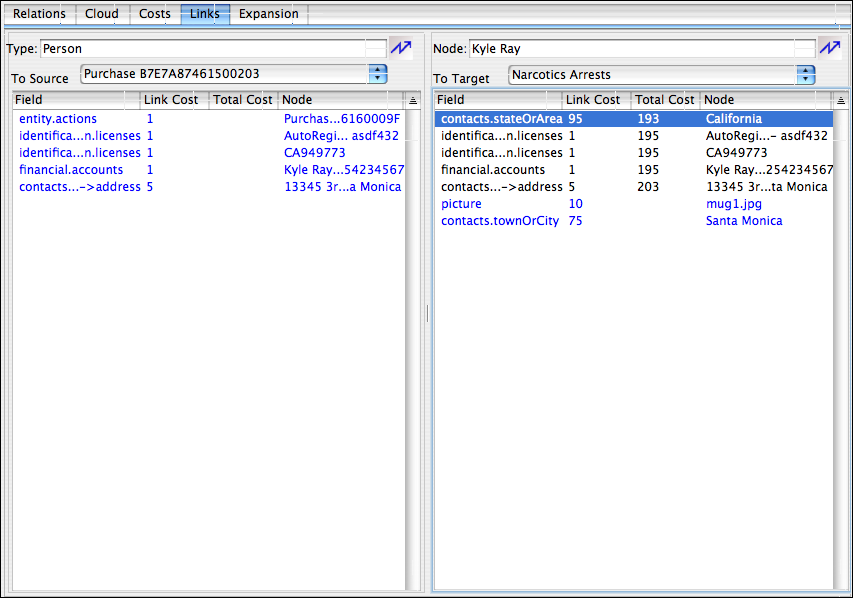
Here we see a small snapshot of the connection ‘cloud’ that is building up behind the paths area, in this case just the links passing through the underlying ontology from the ‘Person‘ node ‘Kyle Ray’ between the source and target node. We can see that currently we have upstream links mediated by the ‘##entity.actions‘ (the purchase action), ‘##identification.licenses‘ (the driving license he showed to identify himself – which leads to DMV records – another source that has been mined and integrated), and a couple of others. On the downstream side, we see 7 possible paths to the target, each with a different individual link cost as well as a total cost to reach the target obtained by adding all intermediate link costs. All these links are simply being manifested as part of Mitopia’s underlying Carmot ontology when used to integrate data across multiple different sources using MitoMine™. Unlike conventional link visualizers, the analyst does not have to ‘create’ these links manually in order to see/visualize the connection – the contiguous ontology does it all automatically.
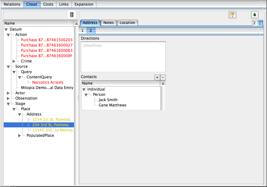
The link to California has been selected above and goes through the ‘#contacts.stateOrArea‘ field of the ontological type ‘Person‘ – that is Kyle Ray lives in California. If we double click the ‘Field’ cell, we are taken immediately to the ‘Cloud’ tab showing the full data for ‘Kyle Ray’ in the invisible cloud behind the visualizer:
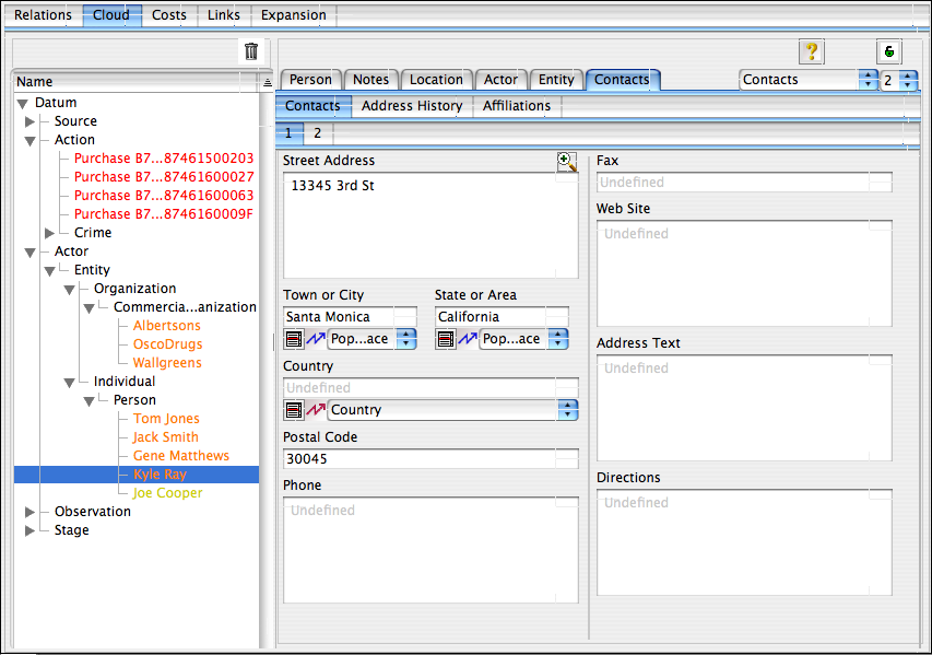
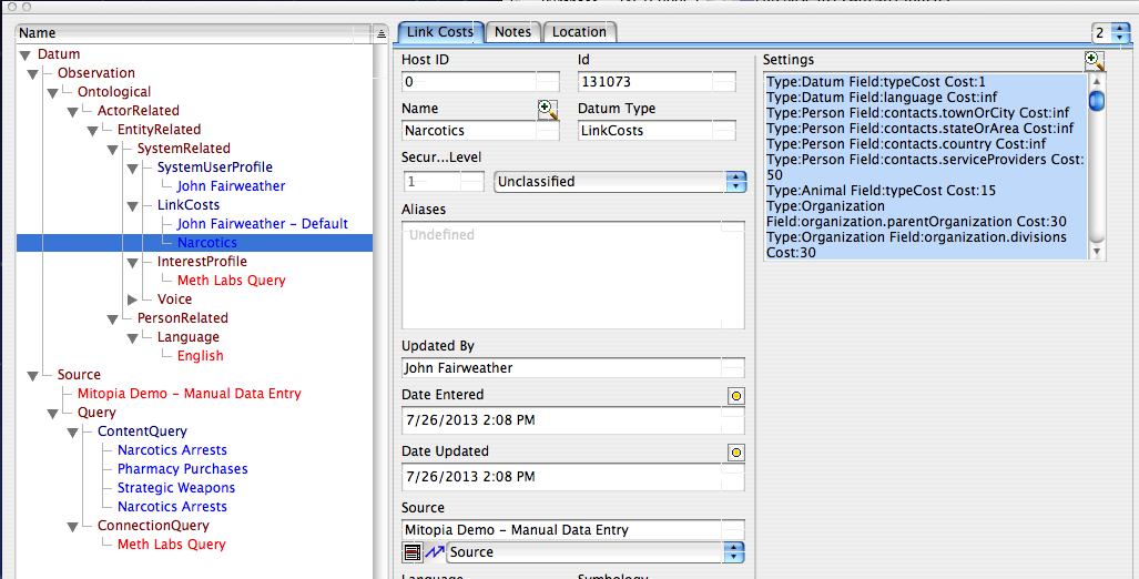
As can be seen, ‘Kyle Ray’ lives at ‘13345 3rd St’ in the City of ‘Santa Monica’ and the State of California. The display of this data is being laid out automatically based on the underlying ontology as described here. Note that the ontology is also driving the layout of the list on the left and in addition the nodes are color coded to indicate how many ‘expansion’ steps they are away from an endpoint (starting with ‘red’ for endpoint, ‘orange’ for first expansion, and so on). This is because every time the user clicks ‘Expand Cloud’, the system takes all the new ontological nodes within the cloud returned from the previous expansion (or initially endpoints) and follows every link field described by the ontology for that type to retrieve a new ‘silver lining’ of nodes not yet explored from the servers. This data is then added to the invisible backing cloud for the visualizer and hooked up automatically by the ontology. It is these ontological links that the system then explores looking for connections. We could have navigated directly to the ‘Costs’ tab which shows the specific links present for the node ‘Kyle Ray’ in the directions of the selected source and target by double clicking the ‘Link Cost’ column from our earlier ‘Links’ tab display, the result would be as follows:
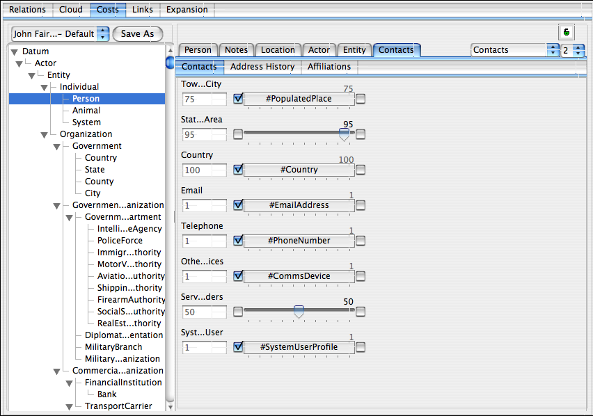
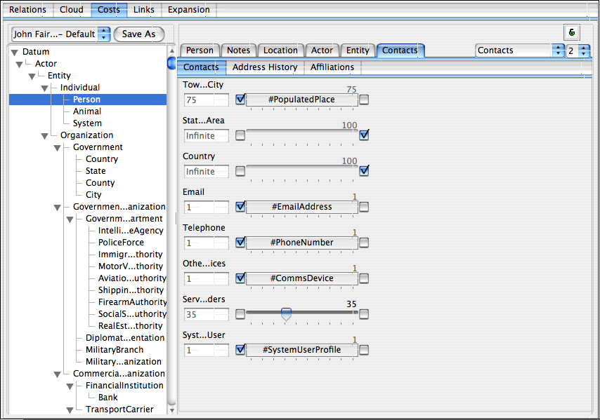
In this (also auto-generated) display, we see for each field within the ‘contacts‘ area of the Kyle Ray node’s type (i.e., Person) a set of sliders indicating the individual link path cost involved in following the link involved. Those links shown checked to the left are costs inherited from the type shown in the center (that is the cost to follow the ‘#townOrCity‘ link is inherited from the type ‘PopulatedPlace‘ which is 75). We can alter the checkboxes or move the sliders for any field in any type within the ontology (including of course ‘inherited’ costs) in order to specify for this particular problem what types of links are important. The links that are important for one type of question are very likely quite different for another type of question, so it is important that we can tune all links specifically for the problem at hand. With more than 100 different types of number of adjustments for every single type that can be combined with inheritance, there is literally an infinite number of ways to tune the link costs for a given problem. In the example below, I have set the costs for the ‘#contacts.stateOrArea‘ field that was causing our unwanted shortest path to ‘infinite’ by checking the checkbox to the right; I have done the same for the ‘#country‘ field which is clearly also not important in this case. Finally I tweaked the slider for ‘##contacts.serviceProviders‘ (i.e., companies that the person relies on for services e.g., water, electricity, phone, etc.) mainly just to show how this looks in the UI.
If we then go back to the ‘Relations’ tab, click the ‘Reset’ button and then expand afresh to the same state, we now see (see screen shot below) that the shortest path through ‘#contacts.stateOrArea‘ has been eliminated and the fourth purchase is no longer considered to be significantly connected to a narcotics offender. This cost adjustment is thus our first step to training the link visualizer what kind of connections we care about in this case.
 Of course with so many potential connections, we probably have many more cycles of this process to go through before we get exactly the significant purchases we want and no others. For example lets examine the path that passes through ‘234 3rd St, Pomona’. Ontologically speaking, this is an ‘Address‘ which among other things is a kind of ‘Place‘ at which you can likely find one or more entities of interest. We can see from the screen shot to the right that both ‘Jack Smith’ and ‘Gene Mathews’ live at this address, that is they are room mates (according to the DMV records). Perhaps Jack has sent Gene to buy his PSE for him and so this is another kind of link that we want to consider important in this case.
 In contrast however, if we look at the link through the City of Pomona that connects ‘Tom Jones’ to ‘Jack Smith’, we see that it passes through the ‘#contacts.townOrCity‘ field with a cost of 75. Again the fact that these two live in the same City is not significant in this particular case, so we should adjust this cost the inhibit finding this link as a lowest cost path.
This cycle will repeat through many potential linking fields. For example the DMV is the same government organization that granted all the driving licenses and eventually this connection may float to the top as a shortest possible path. Same goes for a host of other link types.
After cycling through adjusting various costs and expanding the cloud a number of additional steps, we will hopefully reach a point where the cloud does not expand any further, and the only paths we have shown are the ones that we wish to be considered significant, all others are considered irrelevant. This situation is depicted for this simple example data set below:
Here we have expanded four times (i.e., there may be up to 8 degrees of separation between a source and a target), in real data sets, one might expand up to 10 times (i.e., 20 degrees of separation) and have tens of thousands of nodes in the backing cloud containing literally millions of potential connections. You can see that one additional significant link has been found in this data set which is caused by the fact that the DMV record for Kyle Ray (the purchaser) shows that he owns a 1999 Ford Focus (registration ASDF432) in which Joe Cooper (another individual arrested for narcotics) was actually arrested earlier. Clearly then Kyle and Joe probably know each other quite well, even though with this data set we may not know how. This connection is thus significant and may warrant further investigation.
 For the sake of completeness, the content of the ‘Expansion’ tab is shown to the left. In reality what is going on during link analysis is a constant competition between one or more ‘expanders’ and one or more ‘pruners’ that can be registered with the visualizer dynamically and as necessary for the problem at hand. In the example, we only used the most basic of each of these which for the ‘expander’ simply follows ontology-mediated connections, and for the ‘pruner’ simply stops exploring any path once its total cost from an endpoint exceeds an adjustable limit (in this case 150). Clearly without some kind of active pruning, with a universal ontology like Carmot, this kind of link analysis will fall prey to the theory of ‘six degrees of separation‘ which holds that everything and everyone is connected to all others by no more that six steps. In other words without active pruning, after a few expansions, we could well pull the entire world (or at least the entire data set) into the invisible backing cloud. There are a number of other pruning tools provided, and Mitopia® allows custom pruning algorithms to be developed and registered for specific problem domains.
On the expansion side, once again different problems may require specialized expander algorithms to be invoked, and these too can be registered with the generic link analyzer. For example, one might want to register an ‘expander’ that did image recognition on DMV and other pictures looking for an individual whose image was captured in a security camera. If registered, such expanders are invoked automatically (if appropriate) by Mitopia® during the expansion process, and thus the range of problems that can be tackled through this tool is essentially unbounded.
All this is very well you might say, but what has it got to do with asking knowledge-level queries? The answer is that unlike other link analysis systems, what we have been doing above is not just visualization, we have in actually been creating a knowledge-level query as a side effect!
The leap from visualization to knowledge-level query
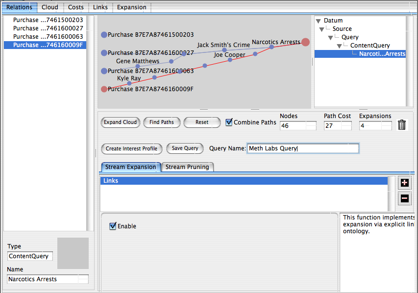
In the screen shot above, the user has dragged the expandable panel at the bottom of the visualizer upwards to reveal additional UI allowing them to save their work as a knowledge level query and optionally also an interest profile. A Mitopia® interest profile is a query that is run automatically and continuously whenever any new data arrives at the servers that match the type specified. When any data matches the the query, the user that created the interest profile is notified. In other words, this single step would allow the police department in our example above to continuously monitor all subsequent PSE purchases and to be notified automatically every time a suspicious purchase occurred. When the user opens the notification that results, the system automatically displays the link analysis diagram that led to the alert so allowing the notified individual to examine the diagram to determine if any additional action is required (which may of course include further tuning of the query to eliminate newly revealed nuisance alerts).
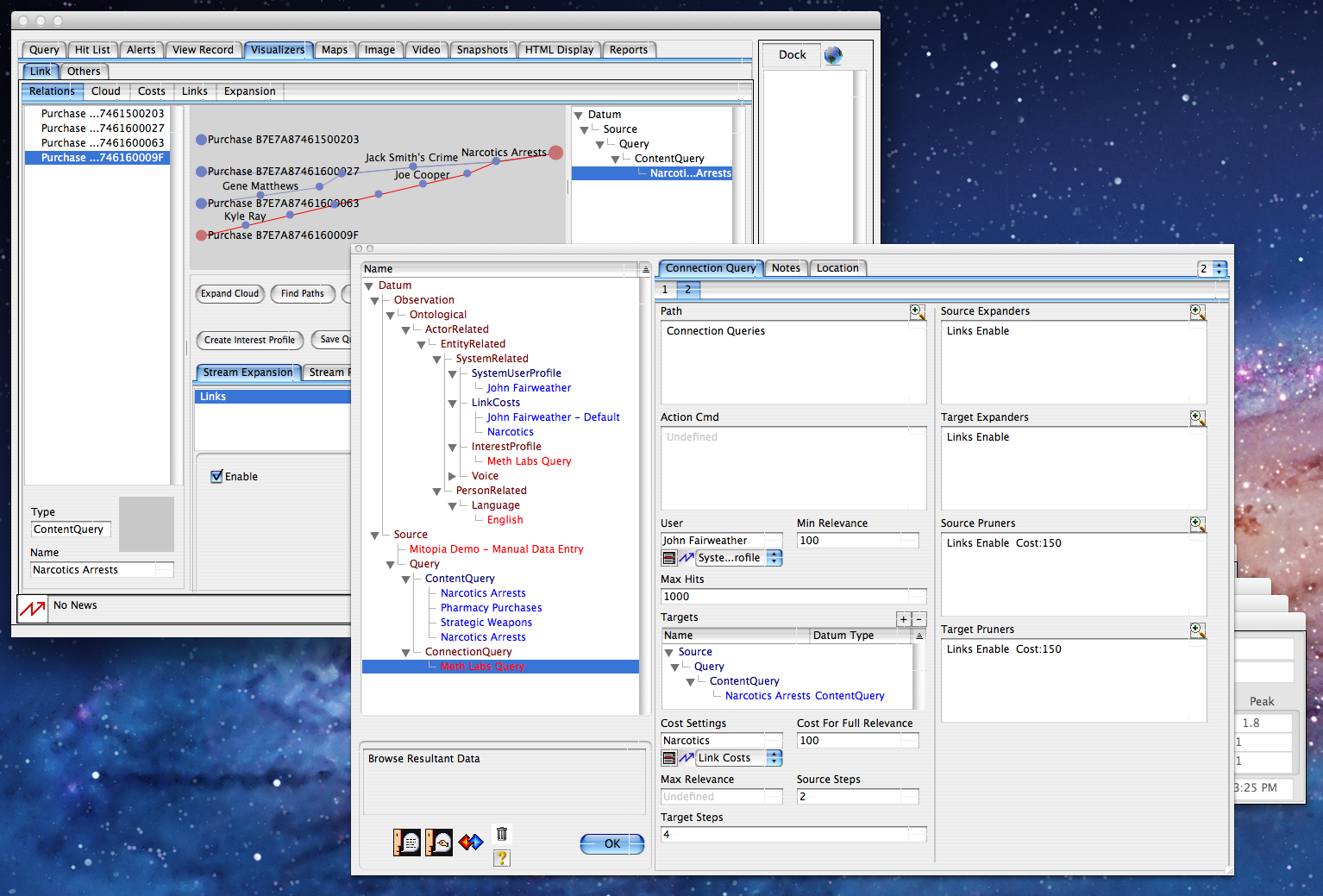
 In the screen shot above, the user has chosen to create an interest profile which like everything else in Mitopia® is described by the ontology itself and thus is auto-displayed and stored/retrieved in exactly the same way as any other ontological type might be. You can see that the ConnectionQuery definition is referenced from the interest profile and contains the details of the ‘target’ node (in this case the ‘Narcotics Arrests’ query) to which the source type data (in this case a subtype of ‘Action‘) should be linked. Note that in addition to allowing embedded queries of all kinds (far more powerful than SQL queries) within the expansion diagram, the ‘filter‘ field of the query allows yet another query (of any type) to be used to filter data to be processed by the connection query. Details of the number of source and target expansion steps as well as the expansion and pruning chains are also specified within the type ‘ConnectionQuery‘. Note also that the specialized set of adjusted costs (type ‘LinkCosts‘) for this query are also saved and referenced via the ontology from the ‘#costSettings‘ field of the query (shown to the right).
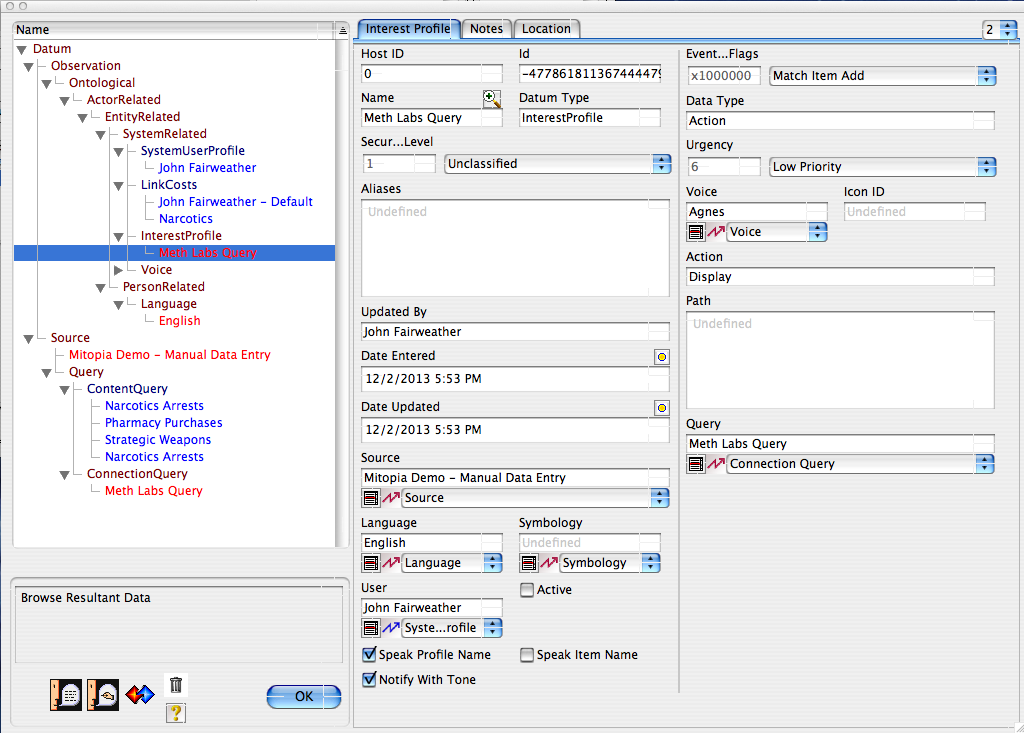
If we look at the interest profile node (shown above), we see that the user has the ability to specify how they want to be notified (and with what urgency), if they want the item name to be spoken and with which voice, and a number of other settings including the actual action that happened to the server data (which defaults to item ‘add’, could also be ‘read’, ‘write’, or ‘delete’ – useful for counter intelligence purposes).
When the user has changed any settings necessary and clicked the ‘OK’ button, the system is now continuously and automatically monitoring all new PSE purchases against the criteria specified and notifies the appropriate users when a significant match occurs. Although we said we wouldn’t go into the details of how the query/interest profile is actually executed at this time, perhaps we can paint at least a high level picture.
 You will note from the screen shot of the ConnectionQuery above that the user has the ability to separately control the number of ‘source’ and ‘target’ expansion steps. For example in a particular case we might choose to set ‘targetSteps‘ to 5 and ‘sourceSteps‘ to 3. When running the query against incoming data as an interest profile, the server performs the target expansion steps just once, caching the results. This in effect creates a fan shaped set of ontological nodes (imagine it like the coral shown to the left) where the shape of the fan is finely tuned to detect a particular kind of ‘significance’ based on the settings made within the link analyzer. What we have is thus a finely tuned web, designed to react to a particular kind of stimulus. This tuned web is then inserted into the incoming data flow, much like a coral would filter debris from ocean currents.
 Now as a new data item of the selected type is ingested, the server takes that item as a nucleus and expands out from it by the number of steps specified in ‘sourceSteps‘. This creates a floating ‘ball’ of ontological connections clustered around the nucleus. The process of executing the query then becomes a matter of checking for connected paths from the floating nucleus to the stem of the coral fan in much the same way we did in the link visualizer (but more optimized). If a path is found with a cost below that specified in ‘maxRelevance‘, the query matches and the nucleus record is a returned as a hit or triggers an interest profile notification.
In summary we can see that through the use of a pervasive and contiguous ontology, Mitopia® allows interactive creation and subsequent execution of knowledge level queries that make current generation database systems and queries look positively primitive. The other half of this puzzle is ensuring that such complex queries execute rapidly.
NOTE:Obviously we have skipped a lot of detail in this initial introduction to the subject of knowledge-level queries. You will find demos involving link analysis based queries in the “Mitopia.demo.m4v” (the same example scenario – go to offset 22:40) and “MitopiaBigData.mov” (go to offset 11:20) videos on the “Videos,demos & papers” page. For a detailed look at other complex query types, see the “MitoipaNoSQL.m4v” video on the same page.